Tracking Visitor Counts before and during COVID-19 Pandemic
Using data provided by SafeGraph, we were able to track the frequency of shoppers for select store brands, and also categorizing the freqeuncy of shopper visits based on their dwell times. Since the start of the pandemic, the dynamics of shopping has changed, where the number of visitors in stores changed once quarantine started. For this analysis, New York City was analyzed.
In [1]:
import pandas as pd
import geopandas as gpd
import json
import numpy as np
import matplotlib.pyplot as plt
from matplotlib.pyplot import figure
Create the Bucket Dwell Time Class
In [2]:
class Bucketed_Dwell_Time:
    def __init__(self, lst):
        self.lst = lst

    def average(self, lst):
        return sum(lst) / len(lst)

    def listSum(self, lst):
        total = 0
        item = 0
        while(item < len(lst)):
            total = total + lst[item]
            item += 1
        return total
    def findMedian(self, lst):
        n = len(lst)
        lst.sort()
        if n % 2 == 0:
            median1 = lst[n//2]
            median2 = lst[n//2 - 1]
            median = (median1 + median2)/2
        else:
            median = lst[n//2]
        return median
    def organizeDwells(self):
        dwell1 = []
        dwell2 = []
        dwell3 = []
        dwell4 = []
        dwell5 = []
        for b in self.lst:
            for k, v in b.items():
                if k == '<5':
                    dwell1.append(v)
                elif k == '5-20':
                    dwell2.append(v)
                elif k == '21-60':
                    dwell3.append(v)
                elif k == '61-240':
                    dwell4.append(v)
                else:
                    dwell5.append(v)
        self.dwell1 = dwell1
        self.dwell2 = dwell2
        self.dwell3 = dwell3
        self.dwell4 = dwell4
        self.dwell5 = dwell5

    def bDwell_avg(self):
        self.organizeDwells()
        bcktDwell_avg = {'<5': self.average(self.dwell1), '5-20': self.average(self.dwell2),
                         '21-60': self.average(self.dwell3),'61-240': self.average(self.dwell4),
                         '>240': self.average(self.dwell5)}
        return bcktDwell_avg
    def bDwell_median(self):
        self.organizeDwells()
        bcktDwell_mdn = {'<5': self.findMedian(self.dwell1), '5-20': self.findMedian(self.dwell2),
                         '21-60': self.findMedian(self.dwell3),'61-240': self.findMedian(self.dwell4),
                         '>240': self.findMedian(self.dwell5)}
        return bcktDwell_mdn
    def bDwell_count(self):
        self.organizeDwells()
        bcktDwell_count = {'<5': self.listSum(self.dwell1), '5-20': self.listSum(self.dwell2),
                           '21-60': self.listSum(self.dwell3),
                           '61-240': self.listSum(self.dwell4), '>240': self.listSum(self.dwell5)}
        return bcktDwell_count
Get Store Data
In [3]:
def getStoreData(store, week):
    getstore = week[week['location_name']== store]
    bucketDwell = getstore['bucketed_dwell_times']
    bucketDwell_list = []
    for v in bucketDwell:
        v = json.loads(v)
        bucketDwell_list.append(v)
    return bucketDwell_list
New York City Data
In [4]:
read = pd.read_csv("NY_week0302.csv")
NY_pre1 = pd.DataFrame(read)
read2 = pd.read_csv("NY_week0309.csv")
NY_pre2 = pd.DataFrame(read2)
read3 = pd.read_csv("NY_week0323.csv")
NY_post1 = pd.DataFrame(read3)
read4 = pd.read_csv("NY_week0330.csv")
NY_post2 = pd.DataFrame(read4)

store_list = ['McDonald\'s', 'Target', 'Starbucks', 'Whole Foods Market', 'Trader Joe\'s']
Loop through the store list to get total visitor counts, as average visitor counts.
In [5]:
if __name__ == "__main__":
    week_1_averages = {}
    week_1_count = {}
    for store in store_list:
        dwell = getStoreData(store, NY_pre1)
        d = Bucketed_Dwell_Time(dwell)
        avg = d.bDwell_avg()
        count = d.bDwell_count()
        week_1_averages.update( {store: avg} )
        week_1_count.update({store: count})
    week_2_averages = {}
    week_2_count = {}
    for store in store_list:
        dwell = getStoreData(store, NY_pre2)
        d = Bucketed_Dwell_Time(dwell)
        avg = d.bDwell_avg()
        count = d.bDwell_count()
        week_2_averages.update( {store: avg} )
        week_2_count.update({store: count})
    week_3_averages = {}
    week_3_count = {}
    for store in store_list:
        dwell = getStoreData(store, NY_post1)
        d = Bucketed_Dwell_Time(dwell)
        avg = d.bDwell_avg()
        count = d.bDwell_count()
        week_3_averages.update( {store: avg} )
        week_3_count.update({store: count})
    week_4_averages = {}
    week_4_count = {}
    for store in store_list:
        dwell = getStoreData(store, NY_post2)
        d = Bucketed_Dwell_Time(dwell)
        avg = d.bDwell_avg()
        count = d.bDwell_count()
        week_4_averages.update( {store: avg} )
        week_4_count.update({store: count})
Organize the Data
In [6]:
def dataOrganize(weekList, store):
    FiveMin = []
    TwentyMin = []
    SixtyMin = []
    _240 = []
    GreaterThan240 = []
    for item in weekList:
        for k, v in item.items():
            for i in v.items():
                if k == store:
                    if i[0] == '<5':
                        FiveMin.append(i[1])
                    elif i[0] == '5-20':
                        TwentyMin.append(i[1])
                    elif i[0] == '21-60':
                        SixtyMin.append(i[1])
                    elif i[0] == '61-240':
                        _240.append(i[1])
                    else:
                        GreaterThan240.append(i[1])
    output = {'<5': FiveMin, '5-20': TwentyMin, '21-60': SixtyMin, '61-240': _240, '>240': GreaterThan240}
    return output
In [7]:
week_list = [week_1_averages, week_2_averages, week_3_averages, week_4_averages]
organizedData = {}
for store in store_list:
    organizedData.update({store: dataOrganize(week_list, store)})
Define a function that creates a grouped histogram
- Used for looping through the store list.
- The Histogram output will show the distrubtion over the 4 week period of New York City
In [8]:
def groupHistogram(store, data, txtInput):
    for k, v in data.items():
        if k == store:
            for i in v.items():
                if i[0] == '<5':
                    bar1 = i[1]
                if i[0] == '5-20':
                    bar2 = i[1]
                if i[0] == '21-60':
                    bar3 = i[1]
                if i[0] == '61-240':
                    bar4 = i[1]
                else:
                    bar5 = i[1]
    barGroups = [bar1, bar2, bar3, bar4, bar5]
    groupNames = ['<5', '5-20', '21-60','61-240','>240']
    df = pd.DataFrame(barGroups, index = groupNames, columns = ['March 2nd - March 8th', 'March 9th - March 15th', 'March 23rd - March 29th', 'March 30th to April 5th'])
    colorScheme = ['#63a02c', '#b2df8a', '#1f78b4', '#43a0df' ]
    ax = df.plot.bar(rot=0, figsize=(15,10), zorder = 5, color = colorScheme, edgecolor = "white", fontsize = 20)
    plt.grid(axis='y', linestyle='--', linewidth=0.8)
    plt.xlabel('Dwell Time (Minutes)',size = 25)
    plt.ylabel(txtInput+' Number of  Visitors', size = 25)
    plt.title("New York City: "+ txtInput +" Number of Visitors by Dwell Time at "+store, size = 20)
    plt.legend(loc=1, prop={'size': 18})
    plt.savefig('NewYorkCity_'+store+'_'+txtInput+'.png')
Export the average number of visitors by dwell time at each store brand
In [9]:
# Remember - store_list = ['McDonald\'s', 'Target', 'Starbucks', 'Whole Foods Market', 'Trader Joe\'s','Walgreens','CVS','7-Eleven']
for s in store_list:
    groupHistogram(s, organizedData, "Average")
Overall, you can see a difference in visitors in the later two weeks compared to the first two weeks. For the bucketed dwell time of over 240 minutes, it is suggested that some of that data can be from employees who work at that brand store.
Export the total count of visitors by dwell time at each store brand
In [10]:
wkCount_list = [week_1_count, week_2_count, week_3_count, week_4_count]
countData = {}
for store in store_list:
    countData.update({store: dataOrganize(wkCount_list, store)})
In [11]:
for s in store_list:
    groupHistogram(s, countData, "Total")
Just like the results for average visitors, the results show a similar trend for total count of visitors.
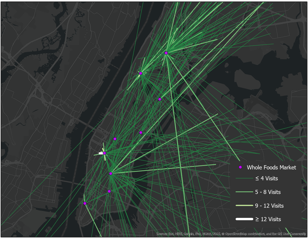
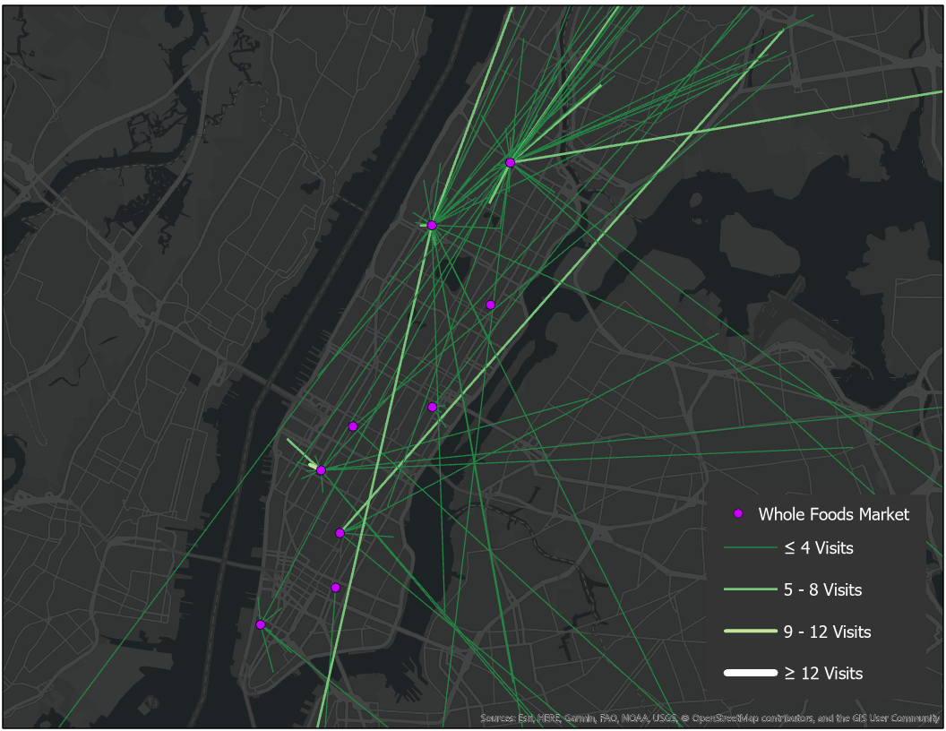
Map out the frequency of store visits before and during the pandemic lockdown. To do this, we got the XY centroid coordinates in the visitor's home U.S. Census Block Group. Once this was retrieved, we created lines from the visitor's home Census Block Group, to the store's XY location.
In [12]:
import shapely
import ast
getFrequency function calculates the total visitors based on store brand and which two week periods they were put in.
In [13]:
def getFrequency(wk1,wk2):
    wk1_visit_cbg = []
    wk1_visit_cbg_count = []
    wk1_poi = []
    wk1_brand_list = []
    wk2_visit_cbg = []
    wk2_visit_cbg_count = []
    wk2_poi = []
    wk2_brand_list = []
    table1 = pd.DataFrame(columns = ['brand','poi_cbg','visitor_cbg'])
    table1['brand'] = wk1['brands']
    table1['poi_cbg'] = wk1['poi_cbg']
    visit_count1 = wk1['visitor_home_cbgs']
    table1['visitor_cbg'] = wk1['visitor_home_cbgs']
    for index, row in table1.iterrows():
        visits = row['visitor_cbg']
        p = row['poi_cbg']
        b = row['brand']
        visits = ast.literal_eval(visits)
        for k, v in visits.items():
            wk1_visit_cbg.append(k)
            wk1_visit_cbg_count.append(v)
            wk1_poi.append(str(p))
            wk1_brand_list.append(b)
    table1 = pd.DataFrame(columns = ['brand','poi_cbg_wk1','visitor_cbg_wk1','visitor_count_wk1'])
    table1['brand'] = wk1_brand_list
    table1['poi_cbg_wk1'] = wk1_poi
    table1['visitor_cbg_wk1'] = wk1_visit_cbg
    table1['visitor_count_wk1'] = wk1_visit_cbg_count
    table2 = pd.DataFrame(columns = ['brand','poi_cbg','visitor_cbg'])
    table2['brand'] = wk2['brands']
    table2['poi_cbg'] = wk2['poi_cbg']
    visit_count2 = wk2['visitor_home_cbgs']
    table2['visitor_cbg'] = wk2['visitor_home_cbgs']
    for index, row in table2.iterrows():
        visits = row['visitor_cbg']
        p = row['poi_cbg']
        b = row['brand']
        visits = ast.literal_eval(visits)
        for k, v in visits.items():
            wk2_visit_cbg.append(k)
            wk2_visit_cbg_count.append(v)
            wk2_poi.append(str(p))
            wk2_brand_list.append(b)
    table2 = pd.DataFrame(columns = ['brand','poi_cbg_wk2','visitor_cbg_wk2','visitor_count_wk2'])
    table2['brand'] = wk2_brand_list
    table2['poi_cbg_wk2'] = wk2_poi
    table2['visitor_cbg_wk2'] = wk2_visit_cbg
    table2['visitor_count_wk2'] = wk2_visit_cbg_count
    table = pd.merge(table1, table2,  how='left', left_on=['poi_cbg_wk1','visitor_cbg_wk1'], right_on = ['poi_cbg_wk2','visitor_cbg_wk2'])
    return table
- getPOICoordinates gets the XY coordinates of the given store.
- getVisitCoordinates gets XY centroid coordinates of the Census Block Group the shopper resides in.
In [14]:
def getPOICoordinates(state, city, df):
    shp = gpd.read_file("shp/"+city+"/"+state+"_BG.shp")
    shp = shp.to_crs('epsg:4326')
    shp = gpd.GeoDataFrame(shp)
    poi_x = []
    poi_y = []
    df['GEOID'] = pd.to_numeric(df['GEOID'], errors='coerce')
    shp['GEOID'] = pd.to_numeric(shp['GEOID'], errors='coerce')
    data = pd.merge(frequency, shp, how='right',on = 'GEOID')
    for index, row in data.iterrows():
        poi_x.append(row['geometry'].centroid.x)
        poi_y.append(row['geometry'].centroid.y)
    data['poi_x'] = poi_x
    data['poi_y'] = poi_y
    del data['ANY UNNECESSARY FIELDS']
    return data

def getVisitCoordinates(state, city, df):
    shp = gpd.read_file("shp/"+city+"/"+state+"_BG.shp")
    shp = shp.to_crs('epsg:4326')
    shp = gpd.GeoDataFrame(shp)
    visit_x = []
    visit_y = []
    df['GEOID'] = pd.to_numeric(df['GEOID'], errors='coerce')
    shp['GEOID'] = pd.to_numeric(shp['GEOID'], errors='coerce')
    data = pd.merge(frequency, shp, how='right',on = 'GEOID')
    for index, row in data.iterrows():
        visit_x.append(row['geometry'].centroid.x)
        visit_y.append(row['geometry'].centroid.y)
    data['visit_x'] = visit_x
    data['visit_y'] = visit_y
    del data['ANY UNNECESSARY FIELDS']
    return data
This loops through the list of csv files in order to differentiate the frequency counts before and after quarantine started.
In [ ]:
period = ['pre','post']
for p in period:
    if p == 'pre':
        read = pd.read_csv("Week 1 csv")
        pr1 = pd.DataFrame(read)
        read2 = pd.read_csv("Week 2 csv")
        pr2 = pd.DataFrame(read2)
    if p == 'post':
        read = pd.read_csv("Week 3 csv")
        pr1 = pd.DataFrame(read)
        read2 = pd.read_csv("Week 4 csv")
        pr2 = pd.DataFrame(read2)
    for s in store_list:
        print("Calculating "+s+" in "+c+"...")
        wk1_store = pr1[pr1['brands'] == s]
        wk2_store = pr2[pr2['brands'] == s]
        frequency = getFrequency(wk1_store, wk2_store)
        freq_list = []
        frequency['visitor_count_wk1'] = frequency['visitor_count_wk1'].fillna(0)
        frequency['visitor_count_wk2'] = frequency['visitor_count_wk2'].fillna(0)
        for index, row in frequency.iterrows():
            total = row['visitor_count_wk1'] + row['visitor_count_wk2']
            freq_list.append(int(total))
        frequency['frequency'] = freq_list
        del frequency['visitor_count_wk1']
        del frequency['visitor_count_wk2']
        del frequency['poi_cbg_wk2']
        del frequency['visitor_cbg_wk2']
        del frequency['brand_y']
        frequency = frequency.rename(columns = {"brand_x":"brand","poi_cbg_wk1":"GEOID","visitor_cbg_wk1":"visitor_cbg"})
        frequency = getPOICoordinates(st, c ,frequency)
        frequency = frequency.rename(columns = {"GEOID":"poi_cbg","visitor_cbg":"GEOID"})
        frequency = getVisitCoordinates(st,c,frequency)
        frequency.to_csv('csv file location')
Next is arcpy, only used for ArcGIS Pro
In [ ]:
import arcpy

arcpy.env.overwriteOutput = True

def ExportXYtoLines(state, store, pr, data, output):
    store = store.replace("'","")
    store = store.replace(" ","")
    store = store.replace("-","_")
    XY_output = output + "/"+city+"_"+store+"_"+pr+"_FREQUENCY"
    arcpy.XYToLine_management(data, XY_output, "poi_x", "poi_y", "visit_x", "visit_y", "Geodesic", "visitor_count")
    diss_output = output + "/"+store+"_"+pr
    statistics_fields = ["visitor_count","SUM"]
    diss_fields = ["poi_x", "poi_y", "visit_x", "visit_y"]
    stat_fields = [["visitor_count","SUM"]]
    arcpy.Dissolve_management(XY_output, diss_output, diss_fields ,stat_fields, "SINGLE_PART")
    arcpy.Delete_management(XY_output)
    brand_store_output = output + "/"+store+"_"+pr+"_POINTS"
    arcpy.management.XYTableToPoint(diss_output,brand_store_output,"poi_x", "poi_y")


output = r"Output gdb here"

for p in period:
    for s in store_list:
        csv = ("csv input here")
        ExportXYtoLines(st, s, p, csv, output)
Once doing the code in arcpy, you can analyze and observe the frequency distributions for the first and last two weeks in this analysis. Here, you can find the frequency in the first two weeks is very high, while the later two weeks show less due to the limitations to shopping during the beginnings of quarantine.
Whole Foods Market - First Two Weeks

Whole Foods Market - Second Two Weeks

In [3]:
import os

os.system('jupyter nbconvert --to html NewYork_StoreVisits.ipynb')
Out[3]: